
외로운 Nova의 작업실
지도 학습 - 나이브 베이즈 본문
- 나이브 베이즈
나이브 베이즈는 확률 기반 머신러닝 분류 알고리즘입니다. 나이브 베이즈를 예시를 통해 이해해보겠습니다.
치킨집에서 손님이 주문을 할때 맥주를 주문할지 안할지 예측해보겠씁니다. 이때 다음과 같은 기존 손님들의 주문 내역이 있습니다.
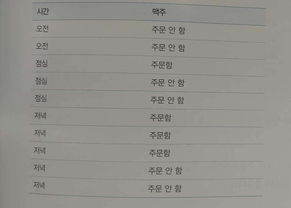
저녁에 손님이 한 명 와서 주문을 합니다. 이 경우 손님이 맥주를 주문할 확률은 조건부 확률이게됩니다. 즉, 저녁에 와서 주문을 할 확률이기 떄문입니다. 이때 나이브 베이즈는 조건부 확률을 계산하는 자신만의 공식으로 계산하게됩니다. 결국 답은 저녁인 5개중에 3개가 주문을 했기때문에 0.6이라는 값을 도출해냅니다. 이런식으로 특징을 많이 뽑아내어 경우의 수를 만들고 나이브 베이즈에 학습시키면 조건부 확률에따라 답을 도출해냅니다.
- 가우시안 나이브 베이즈
가우시안 나이브 베이즈는 하나의 특징에 대한 경우의수가 이산적이 아닌 연속적인 값이고 정규분포를 따르고 있다면 사용하는 알고리즘입니다. 결국 가우시안 나이브 베이즈도 각 데이터 특징에대해서 확률값을 계산하고 결합확률(동시에 발생할 확률)을 계산해서 가장 확률이 높은 한가지를 도출해냅니다. 예제를 통해서 알아보겠습니다.
붓꽃(setosa, versicolor, virginica) 3가지를 꽃받침 길이, 너비, 꽃잎 길이, 너비값 특징을 통해서 분류하는 AI를 만들어보려고합니다. 각각 꽃받침의 길이, 너비, 꽃잎 길이, 너비는 자연현상이기에 정규분포의 형태를 띄게됩니다. 한번 봐보겠습니다.
# 시각화를 위해 pandas를 임포트합니다
import pandas as pd
# iris 데이터는 sklearn에서 직접 로드할 수 있습니다
from sklearn.datasets import load_iris
# sklearn의 train_test_split을 사용하면 라인 한줄로 손쉽게 데이터를 나눌 수 있습니다
from sklearn.model_selection import train_test_split
# Gaussian Naive Bayes로 iris 데이터를 분류하도록 하겠습니다
from sklearn.naive_bayes import GaussianNB
# 분류 성능을 측정하기 위해 metrics와 accuracy_score를 임포트합니다
from sklearn import metrics
from sklearn.metrics import accuracy_score

# iris 데이터를 불러옵니다
dataset = load_iris()
# pandas의 데이터프레임으로 데이터를 저장합니다
df = pd.DataFrame(dataset.data, columns=dataset.feature_names)
# 분류값을 데이터프레임에 저장합니다
df['target'] = dataset.target
# 숫자인 분류값을 이해를 돕기위해 문자로 변경합니다
df.target = df.target.map({0:"setosa", 1:"versicolor", 2:"virginica"})
# 데이터를 확인해봅니다
df.head()

# 분류값 별로 데이터프레임을 나눕니다
setosa_df = df[df.target == "setosa"]
versicolor_df = df[df.target == "versicolor"]
virginica_df = df[df.target == "virginica"]

ax = versicolor_df['sepal length (cm)'].plot(kind='hist')
versicolor_df['sepal length (cm)'].plot(kind='kde',
                                        ax=ax,
                                        secondary_y=True,
                                        title="versicolor sepal length",
                                        figsize = (8,4))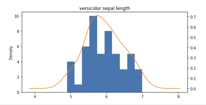
versicolor 꽃받침의 길이 분포를 보면 정규 분포형태를 띄고있음을 알 수 있습니다.
이제 데이터를 학습하고 테스트해보겠습니다.
# 20%를 테스트 데이터로 분류합니다
X_train,X_test,y_train,y_test=train_test_split(dataset.data,dataset.target,test_size=0.2)
# 학습데이터로 모델을 학습합니다
model = GaussianNB()
model.fit(X_train, y_train)

# 테스트 데이터로 모델을 테스트합니다
expected = y_test
predicted = model.predict(X_test)
print(metrics.classification_report(y_test, predicted))
accuracy_score(y_test, predicted)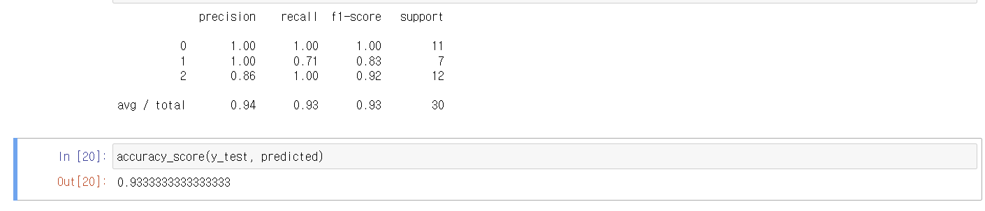
정확도가 0.93으로 높은것을 확인할 수 있습니다.
- 베르누이 나이브 베이즈
베르누이 나이브 베이즈는 이진(binary) 특성을 다루는데 사용됩니다. 이는 주로 문서 분류와 같은 텍스트 데이터에서 단어의 존재 또는 부재를 나타내는 특성에 적용됩니다. 즉, 존재할 확률을 사용해서 분류하게됩니다. 따라서 스팸 메일을 분석할때 스팸 메일에서 자주 발견되는 단어를 분류하고 어떤 단어가 존재하는지에 따라서 스팸 메일인지 아닌지 분류할때 사용할 수 있습니다. 한번 베르누이 나이브 베이즈 알고리즘으로 스팸 메일을 분류하는 AI를 만들어보겠습니다.
import numpy as np
import pandas as pd

# 베르누이 나이브베이즈를 위한 라이브러리를 임포트합니다
from sklearn.feature_extraction.text import CountVectorizer
from sklearn.naive_bayes import BernoulliNB

# 모델의 정확도 평가를 위해 임포트합니다
from sklearn.metrics import accuracy_score

email_list = [
                {'email title': 'free game only today', 'spam': True},
                {'email title': 'cheapest flight deal', 'spam': True},
                {'email title': 'limited time offer only today only today', 'spam': True},
                {'email title': 'today meeting schedule', 'spam': False},
                {'email title': 'your flight schedule attached', 'spam': False},
                {'email title': 'your credit card statement', 'spam': False}
             ]
df = pd.DataFrame(email_list)

df['label'] = df['spam'].map({True:1,False:0})

# 학습에 사용될 데이터와 분류값을 나눕니다
df_x=df["email title"]
df_y=df["label"]
베르누이 나이브베이즈의 입력 데이터는 고정된 크기의 벡터로써, 0과 1로 구분된 데이터이여야 합니다.
sklearn의 CountVectorizer를 사용하여 쉽게 구현할 수 있습니다.
CountVectorizer는 입력된 데이터(6개의 이메일)에 출현된 모든 단어의 갯수만큼의 크기의 벡터를 만든 후,
각각의 이메일을 그 고정된 벡터로 표현합니다.
binary=True를 파라미터를 넘겨줌으로써, 각각의 이메일마다 단어가 한번 이상 출현하면 1, 출현하지 않을 경우 0으로 표시하게 합니다.
cv = CountVectorizer(binary=True)
x_traincv=cv.fit_transform(df_x)
이렇게 하면 email_list에서 17개의 단어를 발견하게됩니다.
cv.get_feature_names()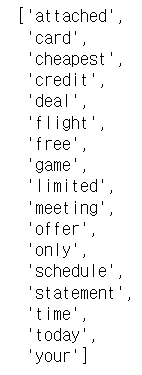
이제 각 email_list가 어떻게 표현되는지 봐보겠습니다.
encoded_input=x_traincv.toarray()
encoded_input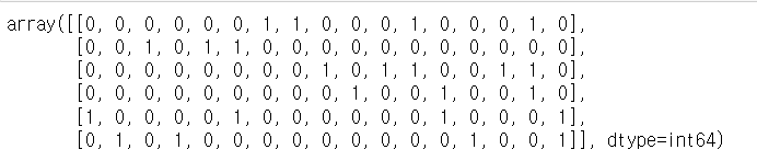
첫번째 행에서는 free, game, only, today 단어가 발견되었다고 각 알맞은 자리에 1(이진 확률)이 표시되는 것을 확인할 수 있습니다. 이제 이걸로 분류해보겠습니다. 즉, 해당 알고리즘으로 학습하게되면 각 단어들에대해서 스팸에대한 조건부확률과 일반메일에 대한 조건부확률을 계산하고 문장에대해서 확률을 계산하게됩니다. 아래는 예시입니다.
스팸 메일 확률을 계산하는 방법은 베르누이 나이브 베이즈에서 조건부 확률을 이용하여 수행됩니다. 각 특성(단어)에 대한 확률을 구하고 이를 조건부 확률의 곱으로 계산합니다. 각 클래스(스팸 또는 일반 메일)에 대한 확률을 계산한 후, 이를 정규화하여 최종적인 확률을 얻습니다.

다음은 간단한 예시를 통해 스팸 메일 확률을 계산하는 과정을 보여줍니다. 간단한 단어들을 이용한 예시입니다.

1. 주어진 메일: "무료 상품 받아보세요. 확인하세요."

2. 사용되는 단어: "무료", "상품", "받아보세요", "확인하세요"

3. 확률 계산:

   - P("무료" | 스팸) = 0.8 (80%의 스팸 메일에 해당 단어가 나타남)
   - P("상품" | 스팸) = 0.7
   - P("받아보세요" | 스팸) = 0.9
   - P("확인하세요" | 스팸) = 0.85

   - P("무료" | 일반) = 0.1 (10%의 일반 메일에 해당 단어가 나타남)
   - P("상품" | 일반) = 0.2
   - P("받아보세요" | 일반) = 0.15
   - P("확인하세요" | 일반) = 0.12

4. 각 클래스에 대한 조건부 확률 계산:

   - P(스팸 | 메일) ∝ P(메일 | 스팸) * P(스팸) = P("무료" | 스팸) * P("상품" | 스팸) * P("받아보세요" | 스팸) * P("확인하세요" | 스팸) * P(스팸)

   - P(일반 | 메일) ∝ P(메일 | 일반) * P(일반) = P("무료" | 일반) * P("상품" | 일반) * P("받아보세요" | 일반) * P("확인하세요" | 일반) * P(일반)

5. 정규화:

   - P(스팸 | 메일) = P(스팸 | 메일) / (P(스팸 | 메일) + P(일반 | 메일))

   - P(일반 | 메일) = P(일반 | 메일) / (P(스팸 | 메일) + P(일반 | 메일))

이렇게 계산된 확률을 비교하여 더 높은 확률을 가진 클래스를 선택하면 됩니다. 여기서 P(스팸)과 P(일반)은 각각 스팸과 일반 메일의 사전 확률을 나타냅니다. 이 예시에서는 간단한 확률 값으로 설명했지만, 훈련 데이터에서 확률을 추정하여 모델을 학습하는 과정이 실제로는 더 복잡합니다.
이제 AI를 학습시켜보겠습니다.
# 학습 데이터로 베르누이 분류기를 학습합니다
bnb = BernoulliNB()
y_train=df_y.astype('int')
bnb.fit(x_traincv,y_train)

# 테스트 데이터 다듬기
test_email_list = [
                {'email title': 'free flight offer', 'spam': True},
                {'email title': 'hey traveler free flight deal', 'spam': True},
                {'email title': 'limited free game offer', 'spam': True},
                {'email title': 'today flight schedule', 'spam': False},
                {'email title': 'your credit card attached', 'spam': False},
                {'email title': 'free credit card offer only today', 'spam': False}
             ]
test_df = pd.DataFrame(test_email_list)
test_df['label'] = test_df['spam'].map({True:1,False:0})
test_x=test_df["email title"]
test_y=test_df["label"]
x_testcv=cv.transform(test_x)

predictions=bnb.predict(x_testcv)

accuracy_score(test_y, predictions)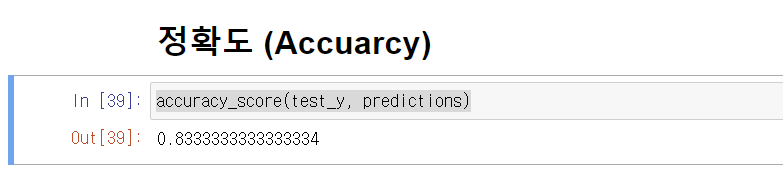
0.83이라는 정확도가 나왔습니다.
- 다항분포 나이브 베이즈
다항 분포 나이브 베이즈는 베르누이 나이브 베이즈와 다르게 빈도수를 계산하게됩니다. 즉, 얼마나 특성이 많이 등장하는지에대한 확률을 가지고 스팸메일로 말하면 스팸메일에 어떤 단어가 얼마나 등장하는지에대한 확률을 가지고 분류를 합니다. 한번 AI를 만들어보겠습니다.
import numpy as np
import pandas as pd
# 다항분포 나이브베이즈를 위한 라이브러리를 임포트합니다
from sklearn.feature_extraction.text import CountVectorizer
from sklearn.naive_bayes import MultinomialNB
# 모델의 정확도 평가를 위해 임포트합니다
from sklearn.metrics import accuracy_score
review_list = [
{'movie_review': 'this is great great movie. I will watch again', 'type': 'positive'},
{'movie_review': 'I like this movie', 'type': 'positive'},
{'movie_review': 'amazing movie in this year', 'type': 'positive'},
{'movie_review': 'cool my boyfriend also said the movie is cool', 'type': 'positive'},
{'movie_review': 'awesome of the awesome movie ever', 'type': 'positive'},
{'movie_review': 'shame I wasted money and time', 'type': 'negative'},
{'movie_review': 'regret on this move. I will never never what movie from this director', 'type': 'negative'},
{'movie_review': 'I do not like this movie', 'type': 'negative'},
{'movie_review': 'I do not like actors in this movie', 'type': 'negative'},
{'movie_review': 'boring boring sleeping movie', 'type': 'negative'}
]
df = pd.DataFrame(review_list)
df['label'] = df['type'].map({"positive":1,"negative":0})
df_x=df["movie_review"]
df_y=df["label"]
cv = CountVectorizer()
x_traincv=cv.fit_transform(df_x)
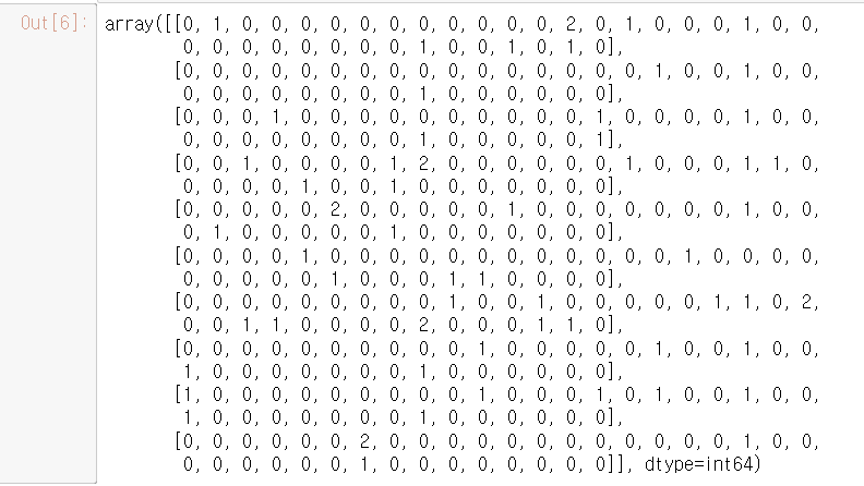
encoded_input=x_traincv.toarray()
encoded_input아래의 행렬에서 볼 수 있듯, 데이터에서 총 37개의 단어가 발견되어, 각각의 영화 리뷰가 37개의 크기를 갖는 벡터로 표현되었습니다.
cv.get_feature_names()
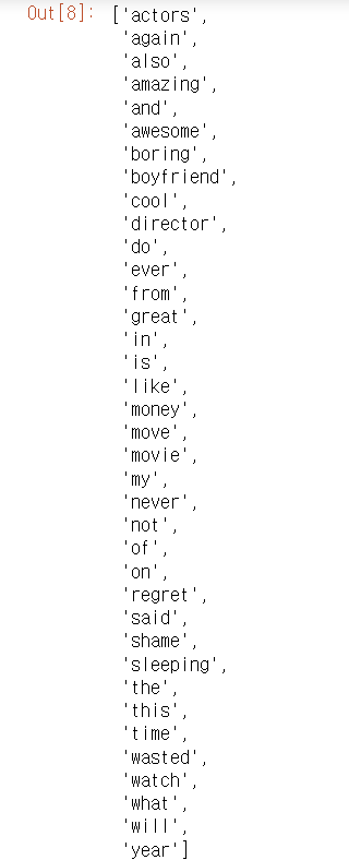
또한 다항분포 나이브베이즈에 사용하기 위해 단어의 빈도수만큼의 수치로 각 단어의 인덱스에 수치가 할당되었습니다.
보게되면 베르누이 나이브 베이즈와 다르게 2가 있는 것을 확인할 수 있습니다. 1은 존재한다가 아닌, 1번 나타났다. 2는 2번 나타났다를 의미하게됩니다.
이제 학습시켜보겠습니다.
# 기존의 데이터로 학습을 진행합니다
mnb = MultinomialNB()
y_train=df_y.astype('int')
mnb.fit(x_traincv,y_train)

test_feedback_list = [
                {'movie_review': 'great great great movie ever', 'type': 'positive'},
                {'movie_review': 'I like this amazing movie', 'type': 'positive'},
                {'movie_review': 'my boyfriend said great movie ever', 'type': 'positive'},
                {'movie_review': 'cool cool cool', 'type': 'positive'},
                {'movie_review': 'awesome boyfriend said cool movie ever', 'type': 'positive'},
                {'movie_review': 'shame shame shame', 'type': 'negative'},
                {'movie_review': 'awesome director shame movie boring movie', 'type': 'negative'},
                {'movie_review': 'do not like this movie', 'type': 'negative'},
                {'movie_review': 'I do not like this boring movie', 'type': 'negative'},
                {'movie_review': 'aweful terrible boring movie', 'type': 'negative'}
             ]
test_df = pd.DataFrame(test_feedback_list)
test_df['label'] = test_df['type'].map({"positive":1,"negative":0})
test_x=test_df["movie_review"]
test_y=test_df["label"]

# 테스트를 진행합니다
x_testcv=cv.transform(test_x)
predictions=mnb.predict(x_testcv)

accuracy_score(test_y, predictions)
정확도가 1인것을 확인할 수 있습니다.
- 차이점
베르누이 나이브 베이즈는 1과 0으로 특성을 나눌 수 있을때 사용해야하고,
다항분포 나이브 베이즈는 1,2,3,4... 여러가지로 특성을 나눌 수 있을때 사용해야합니다.
'AI > machine-learning' 카테고리의 다른 글
| 비지도학습 - 군집화 (0) | 2023.11.04 |
|---|---|
| 앙상블 기법 (0) | 2023.11.03 |
| 지도 학습 - 의사결정 트리 (1) | 2023.10.31 |
| 지도학습 - SVM 서포트 벡터 머신 이론 및 실습 (0) | 2023.10.08 |
| 지도 학습 - knn 알고리즘 이론 및 실습 (1) | 2023.10.07 |


